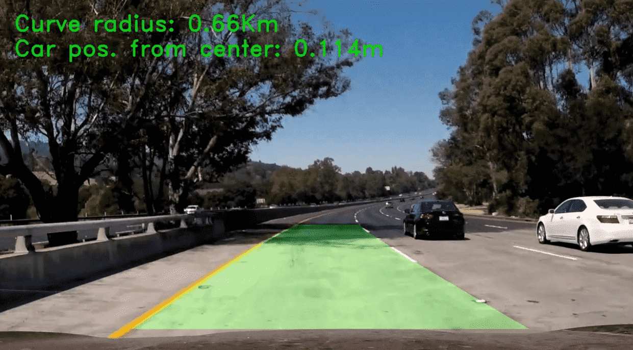
This is the fourth project of self-driving cars engineer nanodegree. In this project we will use advanced techniques and OpenCV to find lane lines.
Advanced Lane Finding Project
The goals / steps of this project are the following:
- Compute the camera calibration matrix and distortion coefficients given a set of chessboard images.
- Apply a distortion correction to raw images.
- Use color transforms, gradients, etc., to create a thresholded binary image.
- Apply a perspective transform to rectify binary image ("birds-eye view").
- Detect lane pixels and fit to find the lane boundary.
- Determine the curvature of the lane and vehicle position with respect to center.
- Warp the detected lane boundaries back onto the original image.
- Output visual display of the lane boundaries and numerical estimation of lane curvature and vehicle position.
My project includes the following files:
- project.ipynb containing all the code.
- project_video_output.mp4 which shows a working example.
- writeup.md/README.md summarizing the results.
This project has 2 parts:
- Define step by step the image processing.
- Define a complete pipeline to process videos.
I splitted the first part of the project in 7 steps:
- Camera calibration
- Distortion correction
- Perspective transformation
- Color/Gradient threshold
- Lane lines detection
- curvature and car position measurement
- Drawing lane lines in original image
Pipeline for a Image
1. Camera Calibration
In this step I used the chessboard images provided in camera_cal folder. First, I tested finding chessboard corners for all images,
# prepare object points, like (0,0,0), (1,0,0), (2,0,0) ....,(6,5,0)
objp = np.zeros((6*9,3), np.float32)
objp[:,:2] = np.mgrid[0:9,0:6].T.reshape(-1,2)

# Arrays to store object points and image points from all the images.
objpoints = [] # 3d points in real world space
imgpoints = [] # 2d points in image plane.

# Make a list of calibration images
images = glob.glob('./camera_cal/calibration*.jpg')
calibration_output_images = []

# Step through the list and search for chessboard corners
for i, fname in enumerate(images):
    img = cv2.imread(fname)
    gray = cv2.cvtColor(img,cv2.COLOR_BGR2GRAY)

    # Find the chessboard corners
    ret, corners = cv2.findChessboardCorners(gray, (9,6),None)

    # If found, add object points, image points
    if ret == True:
        objpoints.append(objp)
        imgpoints.append(corners)

        # Draw and display the corners
        img = cv2.drawChessboardCorners(img, (9,6), corners, ret)
        cv2.imwrite( "./output_images/calibration_output%d.jpg" % i, img )

    calibration_output_images.append(img)

axs = plot_images(10, 2, (20, 50), calibration_output_images)
which results:
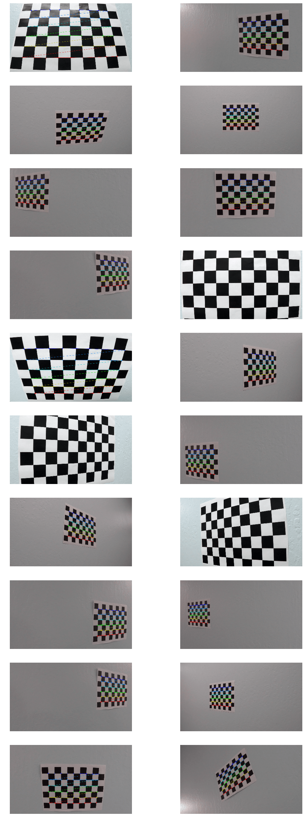
I start by preparing "object points", which will be the (x, y, z) coordinates of the chessboard corners in the world. Here I am assuming the chessboard is fixed on the (x, y) plane at z=0, such that the object points are the same for each calibration image. Thus, objp is just a replicated array of coordinates, and objpoints will be appended with a copy of it every time I successfully detect all chessboard corners in a test image. imgpoints will be appended with the (x, y) pixel position of each of the corners in the image plane with each successful chessboard detection.
For most of the images, the corners were found, and I got as a result objpoints which will be the (x, y, z) coordinates of the chessboard corners in the world. Here I am assuming the chessboard is fixed on the (x, y) plane at z=0, such that the object points are the same for each calibration image. Thus, objp is just a replicated array of coordinates, and objpoints will be appended with a copy of it every time I successfully detect all chessboard corners in a test image. imgpoints will be appended with the (x, y) pixel position of each of the corners in the image plane with each successful chessboard detection..
2. Distortion Correction.
In this step, I used one of the chessboard images to test the distortion correction with this code:
test_image = cv2.imread('./camera_cal/calibration1.jpg')
axs_titles = ['Original', 'Undistorted']

ret, mtx, dist, rvecs, tvecs = cv2.calibrateCamera(objpoints, imgpoints, test_image.shape[0:2], None, None)
undist = cv2.undistort(test_image, mtx, dist, None, mtx)

axs = plot_images(1, 2, (20, 50), [test_image, undist], axs_titles)
which results:

In the previous image we can see that, after applying the distortion correction, the chessboard got effectively undistorted.
The next thing to do is to test it with images from a camera on a car driving through a highway
test_images = glob.glob('./test_images/*.jpg')
undistorted_images=[]
original_images=[]
output_test_images=[]
axs_titles=[]

for i, fname in enumerate(test_images):
    img = cv2.imread(fname)
    img = cv2.cvtColor(img, cv2.COLOR_BGR2RGB)
    output_test_images.append(img)
    original_images.append(img)
    axs_titles.append('Original %d' %int(i+1))

    undist = cv2.undistort(img, mtx, dist, None, mtx)
    undistorted_images.append(undist)
    output_test_images.append(undist)
    axs_titles.append('Undistorted %d' %int(i+1))


axs = plot_images(8, 2, (20, 50), output_test_images, axs_titles=axs_titles, title_fontsize=30)
this code use mtx, dist, None, mtx which we get from cv2.calibrateCamera. These are the results:
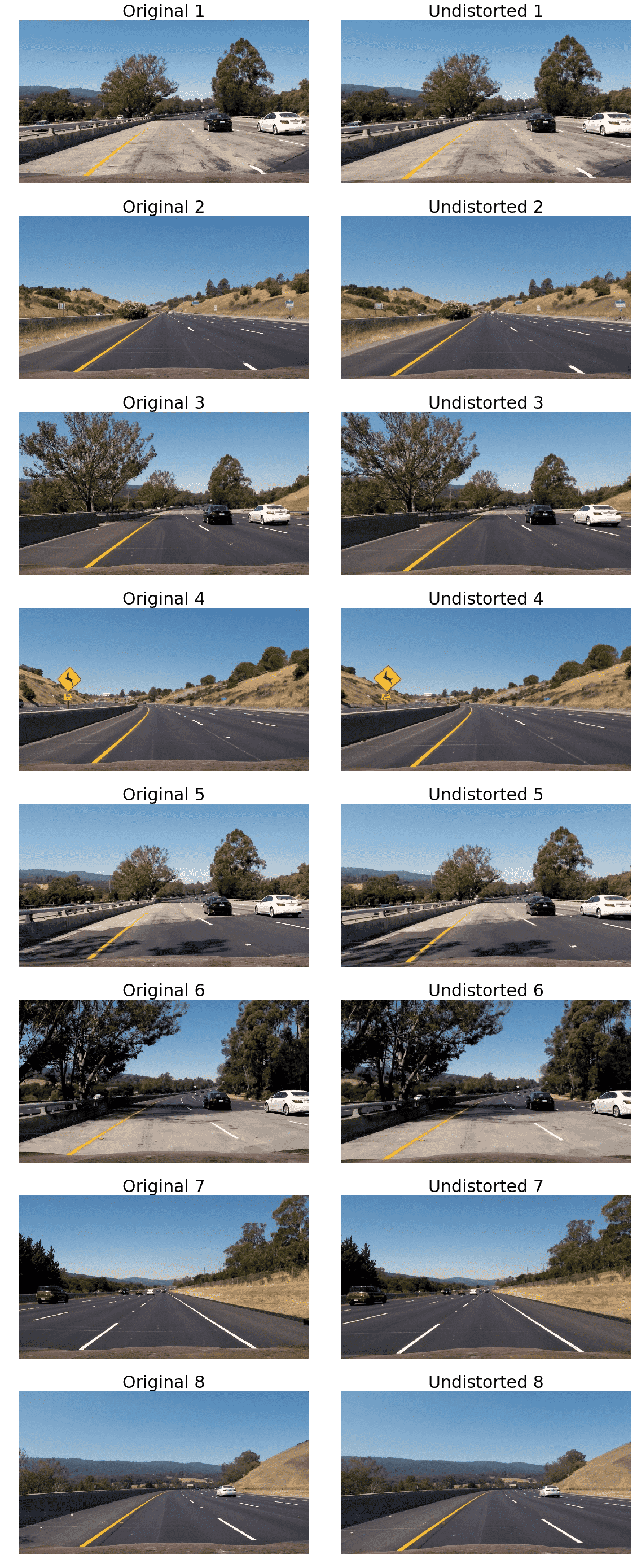
At first, you won't see any difference. But you will see the difference in the car's hood.
3. Perspective Transformation
Once the images are undistorted we apply perspective transformation to see a more accurate view of lane lines.
First, we need to define the area that we want to transform. So, with the help of axis I defined 4 points:
axs_titles = []

for i, image in enumerate(undistorted_images):
    axs_titles.append('Test %d' %int(i+1))

axs = plot_images(4, 2, (20, 50), undistorted_images, axis=True, axs_titles=axs_titles, title_fontsize=30)
x = [580.0, 740.0, 1100.0, 270.0, 580.0]
y = [460.0, 460.0, 670.0, 670.0, 460.0]

for ax in axs:
    ax.plot(x, y, color='#ff1010', alpha=0.5, linewidth=3, solid_capstyle='round', zorder=2)
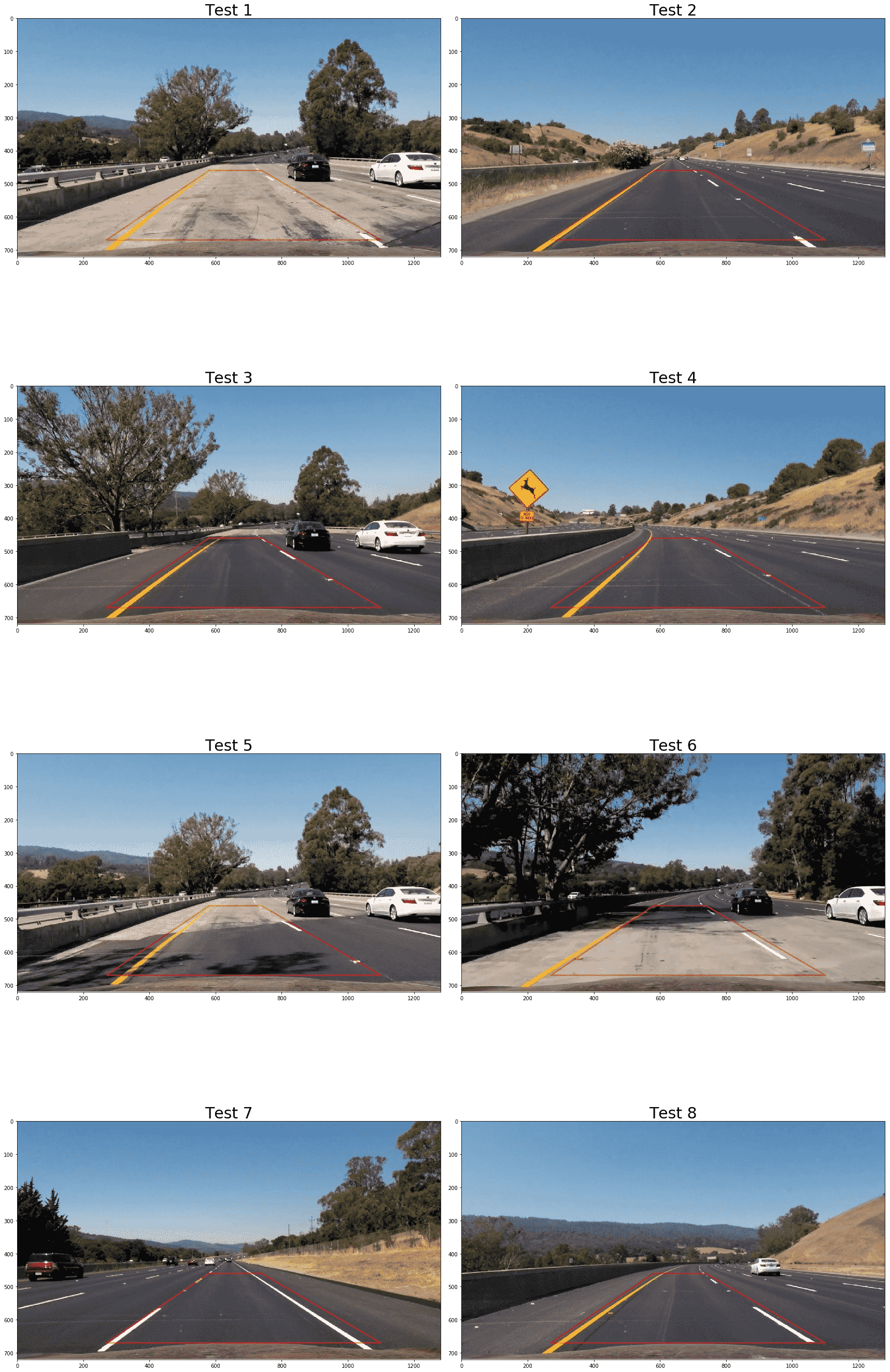
Now we can see the area which will be used for perspective trasnformation.
Next, I defined a warp_image method to use it in the future:
def warp_image(img):
    height, width = img.shape[0:2]

    src = np.float32(
        [
            [580.0, 460.0],
            [740.0, 460.0],
            [1100.0, 670.0],
            [270.0, 670.0],
        ]
    )
    dst = np.float32(
        [
            [200.0, 0],
            [width - 200.0, 0],
            [width - 200.0, height],
            [200.0, height],
        ]
    )

    M = cv2.getPerspectiveTransform(src, dst)
    Minv = cv2.getPerspectiveTransform(dst, src)
    warped = cv2.warpPerspective(img, M, (width, height), flags=cv2.INTER_LINEAR)

    return warped, M, Minv
This resulted in the following source and destination points:
| Source | Destination |
|---|---|
| 580, 460 | 200, 0 |
| 740, 460 | 1080, 0 |
| 1100, 670 | 1080, 720 |
| 270, 670 | 200, 720 |
Then, I applied to test images:
output_test_images = []
warped_images = []
axs_titles = []
Minvs = []

for i, undist in enumerate(undistorted_images):
    output_test_images.append(undist)
    axs_titles.append('Undistorted %d' %int(i+1))

    warped_image, M, Minv = warp_image(undist)
    Minvs.append(Minv)
    warped_images.append(warped_image)
    output_test_images.append(warped_image)
    axs_titles.append('Warped %d' %int(i+1))

axs = plot_images(8, 2, (20, 50), output_test_images, axs_titles=axs_titles, title_fontsize=30)
Finally I got this result:
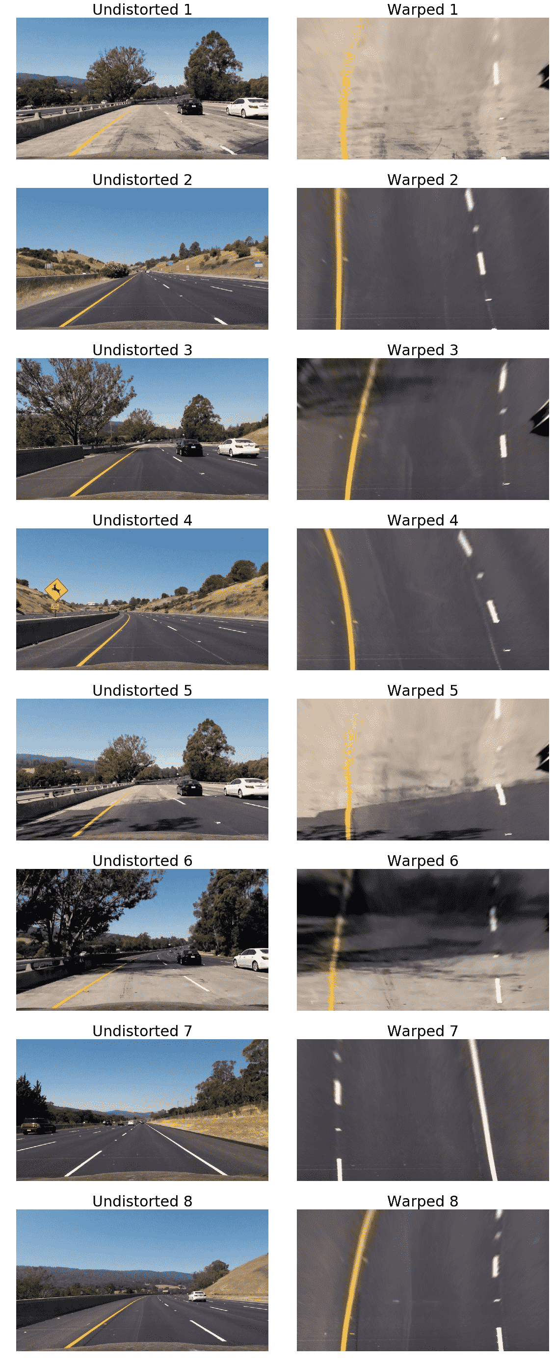
Now you can see the real curvature and distance between each lane lines, and this will focus the algorithm to find only the lane lines that we are interested in.
4. Color/Gradient Threshold
I this step I decided to check different color spaces (RGB and HLS). So, I splitted the image into three channel:
output_test_images = []
axs_titles = []

warped_image = warped_images[5]

# RGB
R = warped_image[:,:,0]
G = warped_image[:,:,1]
B = warped_image[:,:,2]

thresh = (180, 255)
axs_titles.append('R Channel')
output_test_images.append(R)
binary = np.zeros_like(R)

axs_titles.append('G Channel')
output_test_images.append(G)
binary = np.zeros_like(G)

axs_titles.append('B Channel')
output_test_images.append(B)
binary = np.zeros_like(B)

axs = plot_images(1, 3, (20, 50), output_test_images, axs_titles=axs_titles, title_fontsize=15, height_limit=undistorted_images[0].shape[0], width_limit=undistorted_images[0].shape[1], cmap='gray')
# HLS
output_test_images = []
axs_titles = []

warped_image = warped_images[5]
hls_image = cv2.cvtColor(warped_image, cv2.COLOR_RGB2HLS)

H = hls_image[:,:,0]
L = hls_image[:,:,1]
S = hls_image[:,:,2]

axs_titles.append('H Channel')
output_test_images.append(H)

axs_titles.append('L Channel')
output_test_images.append(L)

axs_titles.append('S Channel')
output_test_images.append(S)

axs = plot_images(1, 3, (20, 50), output_test_images, axs_titles=axs_titles, title_fontsize=15, height_limit=undistorted_images[0].shape[0], width_limit=undistorted_images[0].shape[1], cmap='gray')
With these pieces of code we can see an image in three separated channels (R,G,B) or (H,L,S):


In this case we can see that RGB is more understandable, but after testing with videos (2nd part), channels L and S work better than RGB.
So, after testing several times, I decided to use a combination of channels (L and S) and Sobel, Magnitude and Direction thresholds.
def abs_sobel_thresh(img, orient='x', thresh=(0, 255), sobel_kernel=3):
    thresh_min, thresh_max = thresh
    s_thresh = (120, 255)
    l_thresh = (30, 255)

    hls_image = cv2.cvtColor(img, cv2.COLOR_RGB2HLS)

    H = hls_image[:,:,0]
    L = hls_image[:,:,1]
    S = hls_image[:,:,2]

    if orient == 'x':
        sobel = cv2.Sobel(L, cv2.CV_64F, 1, 0, ksize=sobel_kernel)
    else:
        sobel = cv2.Sobel(L, cv2.CV_64F, 0, 1, ksize=sobel_kernel)

    abs_sobel = np.absolute(sobel)
    scaled_sobel = np.uint8(255*abs_sobel/np.max(abs_sobel))

    l_sobel = np.zeros_like(scaled_sobel)
    l_sobel[(scaled_sobel >= thresh_min) & (scaled_sobel <= thresh_max)] = 1

    s_binary = np.zeros_like(S)
    s_binary[(S >= s_thresh[0]) & (S <= s_thresh[1])] = 1

    l_binary = np.zeros_like(L)
    l_binary[(L >= l_thresh[0]) & (L <= l_thresh[1])] = 1

    binary_output = np.zeros_like(l_sobel)
    binary_output[((l_binary == 1) & (s_binary == 1) | (l_sobel==1))] = 1

    return binary_output

def mag_thresh(img, sobel_kernel=3, thresh=(0,255)):

    img = cv2.cvtColor(img, cv2.COLOR_RGB2HLS)[:,:,2]

    sobelx = cv2.Sobel(img, cv2.CV_64F, 1, 0, ksize=sobel_kernel)
    sobely = cv2.Sobel(img, cv2.CV_64F, 0, 1, ksize=sobel_kernel)

    gradmag = np.sqrt(sobelx**2 + sobely**2)

    scale_factor = np.max(gradmag)/255
    gradmag = (gradmag/scale_factor).astype(np.uint8)

    binary_output = np.zeros_like(gradmag)
    binary_output[(gradmag >= thresh[0]) & (gradmag <= thresh[1])] = 1

    return binary_output

def dir_threshold(img, sobel_kernel=3, thresh=(0, np.pi/2)):

    img = cv2.cvtColor(img, cv2.COLOR_RGB2HLS)[:,:,2]

    sobelx = cv2.Sobel(img, cv2.CV_64F, 1, 0, ksize=sobel_kernel)
    sobely = cv2.Sobel(img, cv2.CV_64F, 0, 1, ksize=sobel_kernel)

    abs_sobelx = np.absolute(sobelx)
    abs_sobely = np.absolute(sobely)

    dirs = np.arctan2(abs_sobely, abs_sobelx)

    binary_output = np.zeros_like(dirs)
    binary_output[(dirs >= thresh[0]) & (dirs <= thresh[1])] = 1

    return binary_output

def combined_thresh(img, sobel_kernel=3, abs_thresh=(15,255), _mag_thresh=(15,255), dir_thresh=(0, np.pi/2)):
    gradx = abs_sobel_thresh(img, orient='x', sobel_kernel=sobel_kernel, thresh=abs_thresh)

    mag_binary = mag_thresh(img, sobel_kernel=sobel_kernel, thresh=_mag_thresh)

    dir_binary = dir_threshold(img, sobel_kernel=sobel_kernel, thresh=dir_thresh)

    combined = np.zeros_like(dir_binary)
    combined[((gradx == 1) ) | ((mag_binary == 1) & (dir_binary == 1))] = 1

    return combined
As we can see, in abs_sobel_thresh method I applied sobel threshold to channel L, but I also use L binary and S binary. Finally I combined them
binary_output[((l_binary == 1) & (s_binary == 1) | (l_sobel==1))] = 1
In mag_thresh and dir_threshold I only used S channel.
Finally, I defined a combined_thresh where I combined the different thresholds.
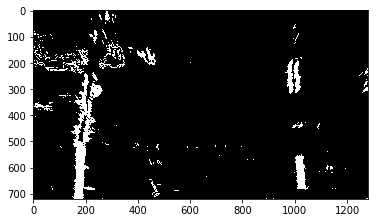
Testing with the same previous image, we get the next binary image:
combined = combined_thresh(warped_images[5], sobel_kernel=3, abs_thresh=(20,255), _mag_thresh=(20,255), dir_thresh=(0, np.pi/2))

plt.imshow(combined, cmap='gray')
5. Lane Lines Detection
Now that we have the binary image, we can used to fine lane lines. But first, we will see a histogram to now how the data behaves.
histogram = np.sum(combined[combined.shape[0]//2:,:], axis=0)
plt.plot(histogram)
And we get:
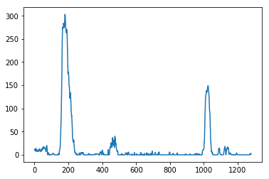
We can see that arround 200px and 1000px are clearly defined the lane lines.
The next thing to do is to find lines through Sliding Windows and Fit a 2nd order Polynomial.
def sliding_window_polyfit(img):
    # Assuming you have created a warped binary image called "binary_warped"
    # Take a histogram of the bottom half of the image
    histogram = np.sum(img[img.shape[0]//2:,:], axis=0)
    # Create an output image to draw on and  visualize the result
    out_img = np.uint8(np.dstack((img, img, img))*255)
    # Find the peak of the left and right halves of the histogram
    # These will be the starting point for the left and right lines
    midpoint = np.int(histogram.shape[0]//2)
    leftx_base = np.argmax(histogram[:midpoint])
    rightx_base = np.argmax(histogram[midpoint:]) + midpoint

    # Choose the number of sliding windows
    nwindows = 9
    # Set height of windows
    window_height = np.int(img.shape[0]//nwindows)
    # Identify the x and y positions of all nonzero pixels in the image
    nonzero = img.nonzero()
    nonzeroy = np.array(nonzero[0])
    nonzerox = np.array(nonzero[1])
    # Current positions to be updated for each window
    leftx_current = leftx_base
    rightx_current = rightx_base
    # Set the width of the windows +/- margin
    margin = 80
    # Set minimum number of pixels found to recenter window
    minpix = 50
    # Create empty lists to receive left and right lane pixel indices
    left_lane_inds = []
    right_lane_inds = []

    # Step through the windows one by one
    for window in range(nwindows):
        # Identify window boundaries in x and y (and right and left)
        win_y_low = img.shape[0] - (window+1)*window_height
        win_y_high = img.shape[0] - window*window_height
        win_xleft_low = leftx_current - margin
        win_xleft_high = leftx_current + margin
        win_xright_low = rightx_current - margin
        win_xright_high = rightx_current + margin
        # Draw the windows on the visualization image
        cv2.rectangle(out_img,(win_xleft_low,win_y_low),(win_xleft_high,win_y_high),(0,255,0), 2)
        cv2.rectangle(out_img,(win_xright_low,win_y_low),(win_xright_high,win_y_high),(0,255,0), 2)
        # Identify the nonzero pixels in x and y within the window
        good_left_inds = ((nonzeroy >= win_y_low) & (nonzeroy < win_y_high) &
        (nonzerox >= win_xleft_low) &  (nonzerox < win_xleft_high)).nonzero()[0]
        good_right_inds = ((nonzeroy >= win_y_low) & (nonzeroy < win_y_high) &
        (nonzerox >= win_xright_low) &  (nonzerox < win_xright_high)).nonzero()[0]
        # Append these indices to the lists
        left_lane_inds.append(good_left_inds)
        right_lane_inds.append(good_right_inds)
        # If you found > minpix pixels, recenter next window on their mean position
        if len(good_left_inds) > minpix:
            leftx_current = np.int(np.mean(nonzerox[good_left_inds]))
        if len(good_right_inds) > minpix:
            rightx_current = np.int(np.mean(nonzerox[good_right_inds]))

    # Concatenate the arrays of indices
    left_lane_inds = np.concatenate(left_lane_inds)
    right_lane_inds = np.concatenate(right_lane_inds)

    # Extract left and right line pixel positions
    leftx = nonzerox[left_lane_inds]
    lefty = nonzeroy[left_lane_inds]
    rightx = nonzerox[right_lane_inds]
    righty = nonzeroy[right_lane_inds]

    # Fit a second order polynomial to each
    left_fit = np.polyfit(lefty, leftx, 2)
    right_fit = np.polyfit(righty, rightx, 2)

    return left_fit, right_fit, left_lane_inds, right_lane_inds, out_img

def visualize_polyfit(img, out_img, left_fit, right_fit, left_lane_inds, right_lane_inds):
    ploty = np.linspace(0, img.shape[0]-1, img.shape[0])
    left_fitx = left_fit[0]*ploty**2 + left_fit[1]*ploty + left_fit[2]
    right_fitx = right_fit[0]*ploty**2 + right_fit[1]*ploty + right_fit[2]

    nonzero = img.nonzero()
    nonzeroy = np.array(nonzero[0])
    nonzerox = np.array(nonzero[1])

    out_img[nonzeroy[left_lane_inds], nonzerox[left_lane_inds]] = [255, 0, 0]
    out_img[nonzeroy[right_lane_inds], nonzerox[right_lane_inds]] = [0, 0, 255]

    plt.figure(figsize = (10,5))
    plt.imshow(out_img)
    plt.plot(left_fitx, ploty, color='yellow')
    plt.plot(right_fitx, ploty, color='yellow')
    plt.xlim(0, 1280)
    plt.ylim(720, 0)
left_fit, right_fit, left_lane_inds, right_lane_inds, out_img = sliding_window_polyfit(combined)

visualize_polyfit(combined, out_img, left_fit, right_fit, left_lane_inds, right_lane_inds)
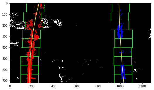
As you can see in the image, I decided to use 9 windows with a margin of 80px which work pretty well.
Once we know where the lines are, we can skip the sliding windows, testing with the same image:
def skip_windows_step(binary_warped, left_fit, right_fit):
    nonzero = binary_warped.nonzero()
    nonzeroy = np.array(nonzero[0])
    nonzerox = np.array(nonzero[1])
    margin = 80
    left_lane_inds = ((nonzerox > (left_fit[0]*(nonzeroy**2) + left_fit[1]*nonzeroy +
    left_fit[2] - margin)) & (nonzerox < (left_fit[0]*(nonzeroy**2) +
    left_fit[1]*nonzeroy + left_fit[2] + margin)))

    right_lane_inds = ((nonzerox > (right_fit[0]*(nonzeroy**2) + right_fit[1]*nonzeroy +
    right_fit[2] - margin)) & (nonzerox < (right_fit[0]*(nonzeroy**2) +
    right_fit[1]*nonzeroy + right_fit[2] + margin)))

    # Again, extract left and right line pixel positions
    leftx = nonzerox[left_lane_inds]
    lefty = nonzeroy[left_lane_inds]
    rightx = nonzerox[right_lane_inds]
    righty = nonzeroy[right_lane_inds]

    # Fit a second order polynomial to each
    left_fit = np.polyfit(lefty, leftx, 2)
    right_fit = np.polyfit(righty, rightx, 2)

    return out_img, left_fit, right_fit, left_lane_inds, right_lane_inds

def visualize_skip_window_step(binary_warped, out_img, left_fitx, right_fitx, left_lane_inds, right_lane_inds):
    margin = 80
    # Generate x and y values for plotting
    ploty = np.linspace(0, binary_warped.shape[0]-1, binary_warped.shape[0])
    left_fitx = left_fit[0]*ploty**2 + left_fit[1]*ploty + left_fit[2]
    right_fitx = right_fit[0]*ploty**2 + right_fit[1]*ploty + right_fit[2]

    # Create an image to draw on and an image to show the selection window
    out_img = np.uint8(np.dstack((binary_warped, binary_warped, binary_warped))*255)
    window_img = np.zeros_like(out_img)

    # Color in left and right line pixels
    nonzero = binary_warped.nonzero()
    nonzeroy = np.array(nonzero[0])
    nonzerox = np.array(nonzero[1])

    out_img[nonzeroy[left_lane_inds], nonzerox[left_lane_inds]] = [255, 0, 0]
    out_img[nonzeroy[right_lane_inds], nonzerox[right_lane_inds]] = [0, 0, 255]

    # Generate a polygon to illustrate the search window area
    # And recast the x and y points into usable format for cv2.fillPoly()
    left_line_window1 = np.array([np.transpose(np.vstack([left_fitx-margin, ploty]))])
    left_line_window2 = np.array([np.flipud(np.transpose(np.vstack([left_fitx+margin, ploty])))])
    left_line_pts = np.hstack((left_line_window1, left_line_window2))
    right_line_window1 = np.array([np.transpose(np.vstack([right_fitx-margin, ploty]))])
    right_line_window2 = np.array([np.flipud(np.transpose(np.vstack([right_fitx+margin, ploty])))])
    right_line_pts = np.hstack((right_line_window1, right_line_window2))

    # Draw the lane onto the warped blank image
    cv2.fillPoly(window_img, np.int_([left_line_pts]), (0,255, 0))
    cv2.fillPoly(window_img, np.int_([right_line_pts]), (0,255, 0))
    result = cv2.addWeighted(out_img, 1, window_img, 0.3, 0)

    plt.figure(figsize = (10,5))
    plt.imshow(result)
    plt.plot(left_fitx, ploty, color='yellow')
    plt.plot(right_fitx, ploty, color='yellow')
    plt.xlim(0, 1280)
    plt.ylim(720, 0)
out_img, left_fit2, right_fit2, left_lane_inds2, right_lane_inds2 = skip_windows_step(combined, left_fit, right_fit)

visualize_skip_window_step(combined, out_img, left_fit2, right_fit2, left_lane_inds2, right_lane_inds2)
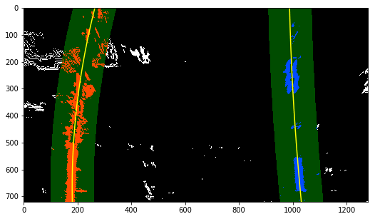
Using the data from the sliding windows, I just searched in a margin around the previous line position.
6. Curvature and Car Position Measurement
I defined two methods calculate the curvature and the car position which will tell us how far the car is from the center of the road:
def measure_curvature(binary_warped, left_lane_inds, right_lane_inds):
    # Define conversions in x and y from pixels space to meters
    ym_per_pix = 30/720 # meters per pixel in y dimension
    xm_per_pix = 3.7/700 # meters per pixel in x dimension

    ploty = np.linspace(0, binary_warped.shape[0]-1, binary_warped.shape[0])
    y_eval = np.max(ploty)

    nonzero = binary_warped.nonzero()
    nonzeroy = np.array(nonzero[0])
    nonzerox = np.array(nonzero[1])

    leftx = nonzerox[left_lane_inds]
    lefty = nonzeroy[left_lane_inds]
    rightx = nonzerox[right_lane_inds]
    righty = nonzeroy[right_lane_inds]

    # Fit new polynomials to x,y in world space
    left_fit_cr = np.polyfit(lefty*ym_per_pix, leftx*xm_per_pix, 2)
    right_fit_cr = np.polyfit(righty*ym_per_pix, rightx*xm_per_pix, 2)

    # Calculate the new radii of curvature
    left_curverad = ((1 + (2*left_fit_cr[0]*y_eval*ym_per_pix + left_fit_cr[1])**2)**1.5) / np.absolute(2*left_fit_cr[0])
    right_curverad = ((1 + (2*right_fit_cr[0]*y_eval*ym_per_pix + right_fit_cr[1])**2)**1.5) / np.absolute(2*right_fit_cr[0])

    return left_curverad, right_curverad

def measure_car_pos(binary_warped, left_fit, right_fit):
    xm_per_pix = 3.7/700
    car_position = binary_warped.shape[1]/2
    height = binary_warped.shape[0]

    left_fit_x = left_fit[0]*height**2 + left_fit[1]*height + left_fit[2]
    right_fit_x = right_fit[0]*height**2 + right_fit[1]*height + right_fit[2]

    lane_center_position = (right_fit_x + left_fit_x) /2

    center_dist = (car_position - lane_center_position) * xm_per_pix

    return center_dist
left_curverad, right_curverad = measure_curvature(combined, left_lane_inds2, right_lane_inds2)

print(left_curverad, 'm', right_curverad, 'm')
car_pos = measure_car_pos(combined, left_fit2, right_fit2)

print(car_pos, 'm')
In the case of the test image:
- Right curvature: 1613.87430742m
- Left curvature: 724.003885913 m
- Car Position: 0.170246440697 m
We can notice that right curvature and left curvature are different numbers, this is because in the previous images we saw that left line and right line are not completely parallel (in this case). In the 2nd part we use an average.
7. Drawing Lane Lines in Original Image
And finally! We draw the results in the original image:
def draw_lines(original_img, binary_img, left_fit, right_fit, Minv):
    ploty = np.linspace(0, binary_img.shape[0]-1, binary_img.shape[0])

    # Create an image to draw the lines on
    warp_zero = np.zeros_like(binary_img).astype(np.uint8)
    color_warp = np.dstack((warp_zero, warp_zero, warp_zero))

    left_fitx = left_fit[0]*ploty**2 + left_fit[1]*ploty + left_fit[2]
    right_fitx = right_fit[0]*ploty**2 + right_fit[1]*ploty + right_fit[2]

    # Recast the x and y points into usable format for cv2.fillPoly()
    pts_left = np.array([np.transpose(np.vstack([left_fitx, ploty]))])
    pts_right = np.array([np.flipud(np.transpose(np.vstack([right_fitx, ploty])))])
    pts = np.hstack((pts_left, pts_right))

    # Draw the lane onto the warped blank image
    cv2.fillPoly(color_warp, np.int_([pts]), (0,255, 0))

    # Warp the blank back to original image space using inverse perspective matrix (Minv)
    newwarp = cv2.warpPerspective(color_warp, Minv, (original_img.shape[1], original_img.shape[0]))
    # Combine the result with the original image
    result = cv2.addWeighted(original_img, 1, newwarp, 0.3, 0)

    return result
new_img = draw_lines(original_images[5], combined, left_fit, right_fit, Minvs[5])
plt.imshow(new_img)
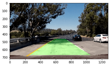
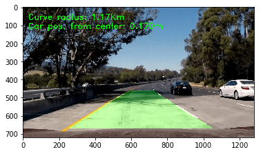
And of course, I also drawed the curvature and car position data:
def draw_curvature_data(img, curv_rad, car_pos):
    font = cv2.FONT_HERSHEY_DUPLEX
    text = 'Curve radius: ' + '{:02.2f}'.format(curv_rad/1000) + 'Km'
    cv2.putText(img, text, (30,70), font, 1.5, (0,255,0), 2, cv2.LINE_AA)

    text = 'Car pos. from center: ' + '{:02.3f}'.format(car_pos) + 'm'
    cv2.putText(img, text, (30,120), font, 1.5, (0,255,0), 2, cv2.LINE_AA)

    return img
final_img = draw_curvature_data(new_img, (left_curverad + right_curverad)/2, car_pos)

plt.imshow(final_img)
Pipeline for Videos
Now it is time to test the previous pipeline on videos.
I defined a Line class to store the lines data along the video.
class Line():
    def __init__(self):
        # was the line detected in the last iteration?
        self.detected = False
        #polynomial coefficients averaged over the last n iterations
        self.best_fit = None
        #polynomial coefficients for the most recent fit
        self.current_fit = []
        #difference in fit coefficients between last and new fits
        self.diffs = np.array([0,0,0], dtype='float')

    def add_best_fit(self, lane_fit, lane_inds):
        if lane_fit is not None:
            if self.best_fit is not None:
                self.diffs = abs(lane_fit - self.best_fit)
            if (self.diffs[0] > 0.001 or self.diffs[1] > 1.0 or self.diffs[2] > 100.) and len(self.current_fit) > 0:
                self.detected = False
            else:
                self.detected = True
                self.px_count = np.count_nonzero(lane_inds)
                self.current_fit.append(lane_fit)
                if len(self.current_fit) > 5:
                    self.current_fit = self.current_fit[len(self.current_fit)-5:]
                self.best_fit = lane_fit
        else:
            self.detected = False
            if len(self.current_fit) > 0:
                self.current_fit = self.current_fit[:len(self.current_fit)-1]
                self.best_fit = np.average(self.current_fit, axis=0)
The add_best_fit is used to update the data inside the class. In every frame, if a line has been found, we check that this one is close to the previous best fit, which is an average of the previous 5 fits.
If the detected line is not a good measure, we delete it, and if it close to the others, we add it to current_fit array, which then will be used to define a new best_fit.
If the detected line is the first one (1st frame), we just added as best_fit
Then I created a process_img method, which will process each frame of the video
def process_img(img):
    original_img = np.copy(img)

    undist = cv2.undistort(original_img, mtx, dist, None, mtx)

    warped_image, M, Minv = warp_image(undist)

    binary_img = combined_thresh(warped_image)

    if not left_line.detected or not right_line.detected:
        left_fit, right_fit, left_lane_inds, right_lane_inds, out_img = sliding_window_polyfit(binary_img)
    else:
        out_img, left_fit, right_fit, left_lane_inds, right_lane_inds = skip_windows_step(binary_img, left_line.best_fit, right_line.best_fit)

    left_line.add_best_fit(left_fit, left_lane_inds)
    right_line.add_best_fit(right_fit, right_lane_inds)

    if left_line.best_fit is not None and right_line.best_fit is not None:
        new_img = draw_lines(original_img, binary_img, left_line.best_fit, right_line.best_fit, Minv)

        left_curverad, right_curverad = measure_curvature(binary_img, left_lane_inds, right_lane_inds)
        car_pos = measure_car_pos(binary_img, left_line.best_fit, right_line.best_fit)

        final_img = draw_curvature_data(new_img, (left_curverad + right_curverad)/2, car_pos)
    else:
        new_img = original_img

    return new_img
In this method basically I check if a best_fit has been found. If not, it use sliding_window_polyfit. But, if it is true it use skip_windows_step. With this data, it updates left_line and right_line with the add_best_fit method.
Finally, it only draw lines and curvature and car position data if there is a best_fit and return the image.
I used the previous code with the project_video.mp4 like this:
left_line = Line()
right_line = Line()

video_output1 = 'project_video_output.mp4'
video_input1 = VideoFileClip('project_video.mp4')
processed_video = video_input1.fl_image(process_img)
%time processed_video.write_videofile(video_output1, audio=False)
Conclusion
Comparing this project with the first Finding Lane Lines Project, this is a much better way to do the job. However, when I tested my code with the challenges videos I saw the next issues:
- Strong changes of color (lines parallel to lane lines) inside the space of lane lines are a problem, because it detects them as lane lines. To fix this, I think that I could add a condition that only allow lines separated by ~300px and not less.
- Working only on HLS color space could be a problem in some cases, I think that it would be better to combine it with another color space like RGB or LAB (I read that it could work better).
- Also, it would be nice to add a condition that only allows almost parallel lines and try to improve the perception transformation.
- For really strong curves, it is really hard to find lane lines. A possible solution could be to use a variable area for perspective transformation that change depending on previous curvature calculation.
As always, I enjoyed it a lot and I already want to see what is comming next.
